The Explainable Ensemble Trees (E2Tree) key idea consists of the definition of an algorithm to represent every ensemble approach based on decision trees model using a single tree-like structure. The goal is to explain the results from the esemble algorithm while preserving its level of accuracy, which always outperforms those provided by a decision tree. The proposed method is based on identifying the relationship tree-like structure explaining the classification or regression paths summarizing the whole ensemble process. There are two main advantages of E2Tree:
- building an explainable tree that ensures the predictive performance of an RF model - allowing the decision-maker to manage with an intuitive structure (such as a tree-like structure).
In this example, we focus on Random Forest but, again, the algorithm can be generalized to every ensemble approach based on decision trees.
Setup
You can install the developer version of e2tree from GitHub with:
install.packages("remotes")
remotes::install_github("massimoaria/e2tree")Warnings
The package is still under development and therefore, for the time being, there are the following limitations:
Only ensembles trained with the randomforest package are supported. Additional packages and approaches will be supported in the future;
Currently e2tree works only in the case ofu classification problems. It will gradually be extended to other problems related to the nature of the response variable: regression, counting, multivariate response, etc.
Example 1: IRIS dataset
In this example, we want to show the main functions of the e2tree package.
Starting from the IRIS dataset, we will train an ensemble tree using the randomforest package and then subsequently use e2tree to obtain an explainable tree synthesis of the ensemble classifier.
# Set random seed to make results reproducible:
set.seed(0)
# Calculate the size of each of the data sets:
data_set_size <- floor(nrow(iris)/2)
# Generate a random sample of "data_set_size" indexes
indexes <- sample(1:nrow(iris), size = data_set_size)
# Assign the data to the correct sets
training <- iris[indexes,]
validation <- iris[-indexes,]
response_training <- training[,5]
response_validation <- validation[,5]
Train an Random Forest model with 1000 weak learners
# Perform training:
rf = randomForest(Species ~ ., data=training, ntree=1000, mtry=2, importance=TRUE, keep.inbag = TRUE, proximity=T)
Here, we create the dissimilarity matrix between observations through the createDisMatrix function
D <- createDisMatrix(rf, data=training)
#>
#> Analized  100  trees
#> Analized  200  trees
#> Analized  300  trees
#> Analized  400  trees
#> Analized  500  trees
#> Analized  600  trees
#> Analized  700  trees
#> Analized  800  trees
#> Analized  900  trees
#> Analized  1000  trees
#dis <- 1-rf$proximity
setting e2tree parameters
setting=list(impTotal=0.1, maxDec=0.01, n=5, level=5, tMax=5)Build an explainable tree for RF
tree <- e2tree(D, training[,-5], response_training, setting)
#> [1] 1
#> [1] 2
#> [1] 3
#> [1] 6
#> [1] 13
#> [1] 12
#> [1] 7
Let’s have a look at the output
tree %>% glimpse()
#> Rows: 7
#> Columns: 19
#> $ node          <dbl> 1, 2, 3, 6, 7, 12, 13
#> $ n             <int> 75, 29, 46, 20, 26, 16, 4
#> $ pred          <chr> "setosa", "setosa", "virginica", "versicolor", "virginic…
#> $ prob          <chr> "0.386666666666667", "1", "0.58695652173913", "0.95", "1…
#> $ impTotal      <dbl> 0.69895205, 0.01628657, 0.58135876, 0.31262187, 0.129637…
#> $ impChildren   <dbl> 0.3628642, NA, 0.2091960, 0.2283824, NA, NA, NA
#> $ decImp        <dbl> 0.33608788, NA, 0.37216271, 0.08423945, NA, NA, NA
#> $ decImpSur     <dbl> 0.24963733, NA, 0.33018530, 0.02263852, NA, NA, NA
#> $ variable      <chr> "Petal.Length", NA, "Petal.Width", "Petal.Length", NA, N…
#> $ split         <dbl> 53, NA, 92, 64, NA, NA, NA
#> $ splitLabel    <chr> "Petal.Length <=1.9", NA, "Petal.Width <=1.7", "Petal.Le…
#> $ variableSur   <chr> "Petal.Width", NA, "Petal.Length", "Petal.Width", NA, NA…
#> $ splitLabelSur <chr> "Petal.Width <=0.6", NA, "Petal.Length <=4.7", "Petal.Wi…
#> $ parent        <dbl> 0, 1, 1, 3, 3, 6, 6
#> $ children      <list> <2, 3>, NA, <6, 7>, <12, 13>, NA, NA, NA
#> $ terminal      <lgl> FALSE, TRUE, FALSE, FALSE, TRUE, TRUE, TRUE
#> $ obs           <list> <1, 2, 3, 4, 5, 6, 7, 8, 9, 10, 11, 12, 13, 14, 15, 16, …
#> $ path          <chr> "", "Petal.Length <=1.9", "!Petal.Length <=1.9", "!Petal…
#> $ pred_val      <dbl> 1, 1, 3, 2, 3, 2, 2
Prediction with the new tree (example on training)
pred <- ePredTree(tree, training[,-5], target="virginica")
#> [1] 1
#> [1] 2
#> [1] 3
#> [1] 4
Comparison of predictions (training sample) of RF and e2tree
table(pred$fit,rf$predicted)
#>
#>              setosa versicolor virginica
#>   setosa         29          0         0
#>   versicolor      0         18         2
#>   virginica       0          0        26
Comparison of predictions (training sample) of RF and correct response
table(rf$predicted, response_training)
#>             response_training
#>              setosa versicolor virginica
#>   setosa         29          0         0
#>   versicolor      0         17         1
#>   virginica       0          2        26
Comparison of predictions (training sample) of e2tree and correct response
table(pred$fit,response_training)
#>             response_training
#>              setosa versicolor virginica
#>   setosa         29          0         0
#>   versicolor      0         19         1
#>   virginica       0          0        26
Variable Importance
rfimp <- rf$importance %>% as.data.frame %>%
  mutate(Variable = rownames(rf$importance),
         RF_Var_Imp = round(MeanDecreaseAccuracy,2)) %>%
  select(Variable, RF_Var_Imp)

V <- vimp(tree, response_training, training[,-5])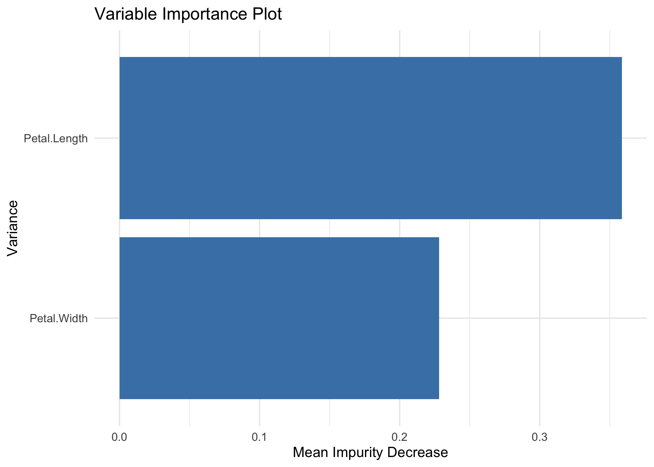

V <- V %>% select(.data$Variable, .data$MeanImpurityDecrease, .data$`ImpDec_ setosa`, .data$`ImpDec_ versicolor`,.data$`ImpDec_ virginica`) %>%
  mutate_at(c("MeanImpurityDecrease","ImpDec_ setosa", "ImpDec_ versicolor","ImpDec_ virginica"), round,2) %>%
  left_join(rfimp, by = "Variable") %>%
  select(Variable, RF_Var_Imp, MeanImpurityDecrease, starts_with("ImpDec")) %>%
  rename(ETree_Var_Imp = MeanImpurityDecrease)

V
#> # A tibble: 2 × 6
#>   Variable     RF_Var_Imp ETree_Var_Imp `ImpDec_ setosa` `ImpDec_ versicolor`
#>   <chr>             <dbl>         <dbl>            <dbl>                <dbl>
#> 1 Petal.Length       0.27          0.36             0.34                 0.02
#> 2 Petal.Width        0.34          0.23            NA                   NA
#> # … with 1 more variable: `ImpDec_ virginica` <dbl>
Comparison with the validation sample
rf.pred <- predict(rf, validation[,-5], proximity = TRUE)

pred_val<- ePredTree(tree, validation[,-5], target="virginica")
#> [1] 1
#> [1] 2
#> [1] 3
#> [1] 4
Comparison of predictions (sample validation) of RF and e2tree
table(pred_val$fit,rf.pred$predicted)
#>
#>              setosa versicolor virginica
#>   setosa         21          0         0
#>   versicolor      0         34         0
#>   virginica       0          0        20
Comparison of predictions (validation sample) of RF and correct response
table(rf.pred$predicted, response_validation)
#>             response_validation
#>              setosa versicolor virginica
#>   setosa         21          0         0
#>   versicolor      0         30         4
#>   virginica       0          1        19
rf.prob <- predict(rf, validation[,-5], proximity = TRUE, type="prob")
roc_rf <- roc(response_validation,rf.prob$predicted[,"virginica"],target="virginica")
roc_rf$auc
#> [1] 0.9873725
Comparison of predictions (validation sample) of e2tree and correct response
table(pred_val$fit,response_validation)
#>             response_validation
#>              setosa versicolor virginica
#>   setosa         21          0         0
#>   versicolor      0         30         4
#>   virginica       0          1        19
roc_res <- roc(response_validation,pred_val$score,target="virginica")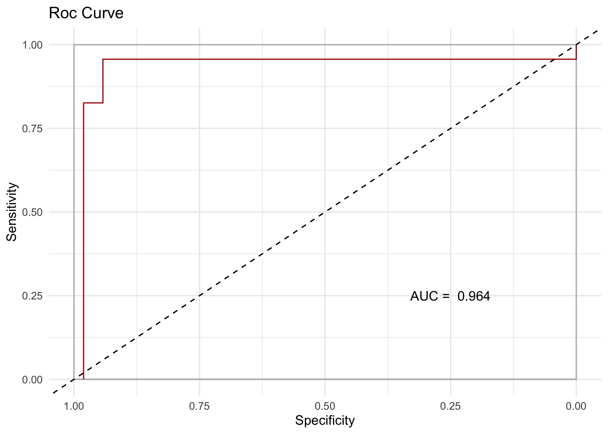
roc_res$auc
#> [1] 0.96395